There are two most important features of google sheets that most people need, but never know how to use it properly. Knowing to use these two features alone, will make you an above average Google Sheets user and allow you to create some pretty advanced charts and customization with your data.
You can save this article for reference, so that you can refer back to it whenever you need to do some advanced data customizations.
In this article we’l go through one of them, VLOOKOUP(). The other one is PIVOT TABLE.
Let’s get started.
VLOOKUP()
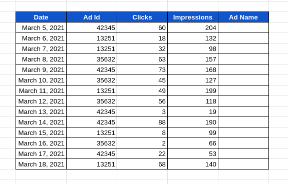
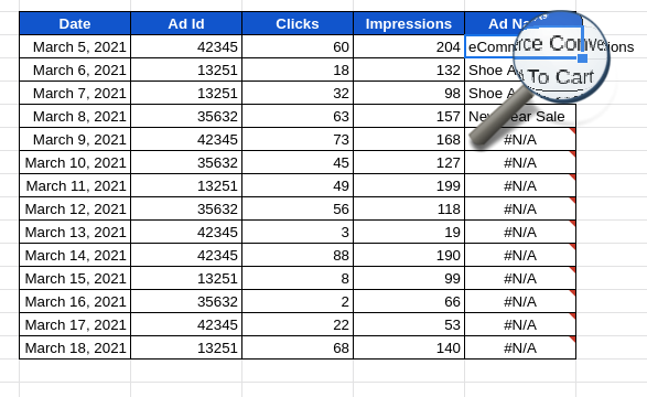
Let’s say you have some ad metrics in your spreadsheet like this image below, but you don’t have the name of the Ads.
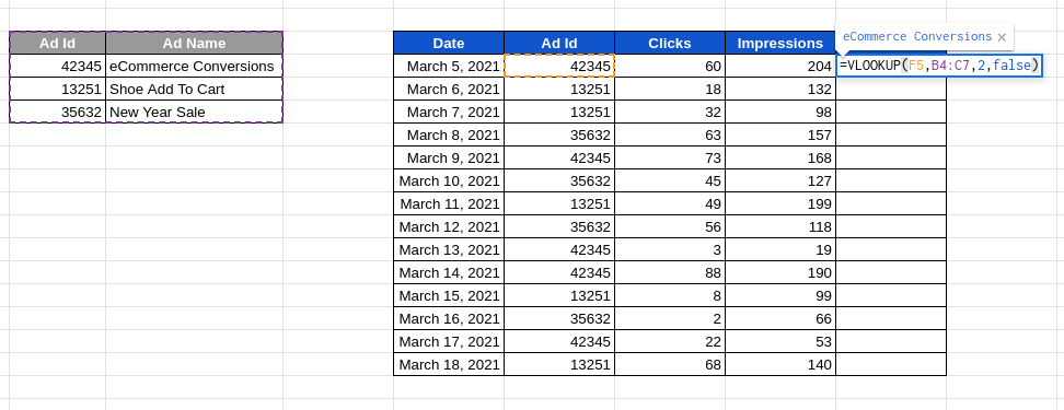
You then went ahead and got the Ad Name from another source into your spreadsheet like below.

How do we merge Ad Name from the new data source in gray table with the blue table? Copy & Paste is one option, but let’s look at an efficient way that will work for many 1000s of rows, the almighty VLOOKUP().
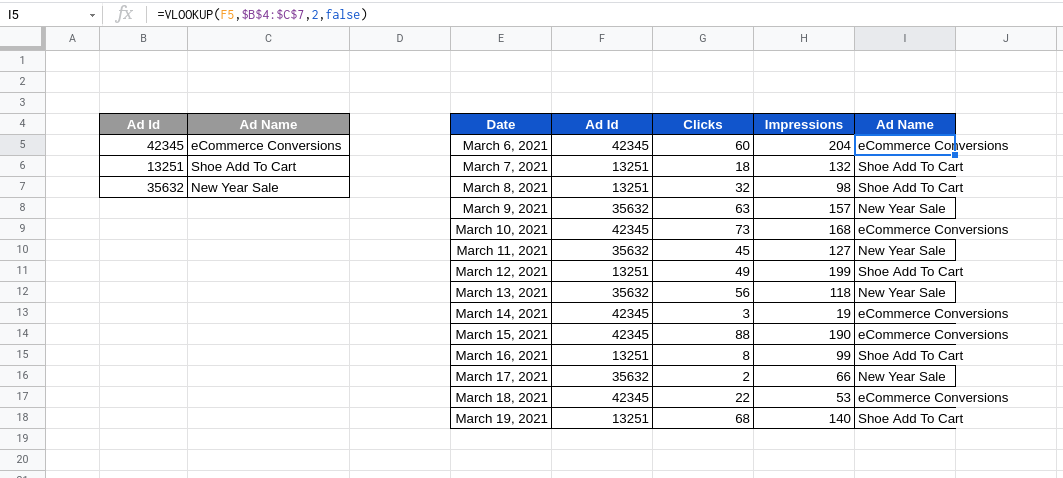
I’ve gone ahead and written the VLOOKUP formula to get Ad Name in our destination table.
You can see that the Ad Name “eCommerce Conversion”, magically pops up on top of our formula, giving a peek into the actual result.
So what’s happening here? Let me explain the VLOOKUP() formula. Here is closer look of the formula we just wrote
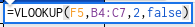
The syntax for VLOOKUP from google is =VLOOKUP(search_key, range, index, [is_sorted])
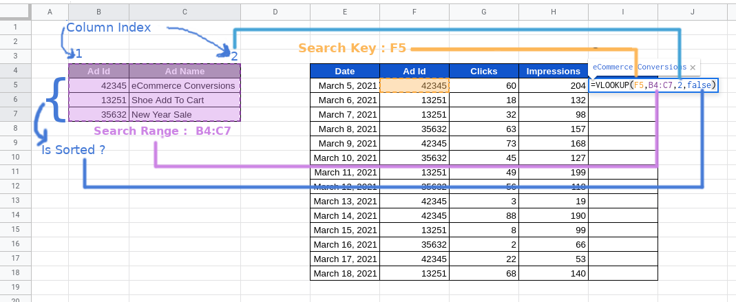
Search Key: It is the unique ID / key that is common between the (destination)blue and (source)gray tables for us to form a link between the two. In our data, “Ad Id” is the common field between these two tables. So we use that as the Search Key, by referencing it with its cell position F5.
Range : It is the source table range that we want to search in; for us it is the gray table, which can be specified as B4:C7
Index : It is the column index within the source table range whose value we want in the destination table’s “Ad Name” column. Since we want “Ad Name” from the source table, we specify 2 as the index, as Ad Name is the second column in our source table range
Is_sorted : It’s always recommended to specify this as false. Setting it as true, expects the tables are already sorted, which if often not the case. Setting the value as true incorrectly will result in incorrect results.
See how our formula references different values in the sheet in the image below
Now that we have our formula for one cell, we can copy paste the formula for all the other rows in the destination table by clicking and dragging the small blue shaded box at the bottom right corner of the formula cell
The formula doesn’t seem to work for all the rows when copied. What could have gone wrong?
When a formula is copied, Google Sheets automatically adjusts the formula to best fit the new place it’s pasted in. But sometimes it needs to be guided properly.
If we look at the formula on cell I9, it is =VLOOKUP(F9,B8:C11,2,false). Here , the Search Key has been correctly adjusted to F9, but the search range has been modified incorrectly. We can correct this by referencing the search range with an absolute range by adding $ before the range column and cell references like this $B$8:C$11.
So the new formula would change to =VLOOKUP(F5,$B$4:$C$7,2,false)and copying just works perfectly.
You can get the full spreadsheet here.
If you are new to Google Sheets, I highly recommend this beginner’s walkthrough of google Sheets by Ben Collins. It’s an amazing resource to learn most of the basic functionalities of Google Sheets.